Book Resume: Introduction to Apache Flink

• Writer: Kostas Tzoumas
• URL: https://cdn2.hubspot.net/hubfs/4757017/Ververica/Docs/Introduction_to_Apache_Flink_book_9781491998809.pdf

Why Apache Flink

In this chapter, we explore what people want to achieve by analyzing streaming data and some of the challenges of doing so at large scale. We also introduce you to Flink and take a first look at how people are using it, including in production.

Consequences of Not Doing Streaming Well

Let’s first look at the consequences of not doing streaming well.

Retail and Marketing

In retail, sales data often comes from website clicks, arriving continuously and unevenly. Using outdated methods can lead to dropped data, delays, or misaggregated results. This can result in inaccurate sales reports, misleading ad billing, and incorrect performance metrics.

The Internet of Things

IoT relies on streaming data for low-latency processing. Sensors send frequent measurements to data centers for real-time applications like updating dashboards, running ML models, and issuing alerts. Inaccurate or delayed processing can compromise these services.

Finance

In finance, real-time detection of anomalous behavior is crucial for fraud prevention. Timely monitoring can catch unusual login patterns or fraudulent transactions, preventing significant losses.

Evolution of Stream Processing Technologies

Background

The disconnect between continuous data production and data consumption in finite batches, while making the job of systems builders easier, has shifted the complexity of managing this disconnect to the users of the systems: the application developers and DevOps teams that need to use and manage this infrastructure.

Apache Storm

To manage this disconnect, some users have developed their own stream processing systems. In the open source space, a pioneer in stream processing is the Apache Storm that started with Nathan Marz and a team at startup BackType (later acquired by Twitter) before being accepted into the Apache Software Foundation.

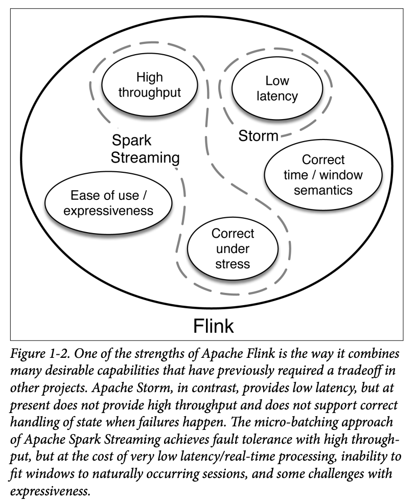
Storm brought the possibility for stream processing with very low latency, but this real-time processing involved tradeoffs:

1. high throughput was hard to achieve
2. Storm did not have exactly-once guarantee for maintaining accurate state

It’s hard to maintain fault-tolerant stream processing that has high throughput with very low latency, but the need for guarantees of accurate state motivated a clever compromise: what if the stream of data from continuous events were broken into a series of small, atomic batch jobs?

Apache Spark Streaming

If the batches were cut small enough—so-called micro-batches—your computation could approximate true streaming. The latency could not quite reach real time, but latencies of several seconds or even subseconds for very simple applications would be possible. This is the approach taken by Apache Spark Streaming, which runs on the Spark batch engine.

More important, with micro-batching, you can achieve exactly-once guarantee of state consistency. If a micro-batch job fails, it can be rerun. This is much easier than would be true for a continuous stream-processing approach.

However, simulating streaming with periodic batch jobs leads to very fragile pipelines that mix DevOps with application development concerns. The time that a periodic batch job takes to finish is tightly coupled with the timing of data arrival, and any delays can cause inconsistent (a.k.a. wrong) results.

The underlying problem with this approach is that time is only managed implicitly by the part of the system that creates the small jobs. Frameworks like Spark Streaming mitigate some of the fragility, but not entirely, and the sensitivity to timing relative to batches still leads to poor latency and a user experience where one needs to think a lot about performance in the application code.

Apache Flink

These tradeoffs between desired capabilities have motivated continued attempts to improve existing processors. When existing processors fall short, the burden is placed on the application developer to deal with any issues that result. With less flexibility and expressivity, development time is slower and operations take more effort to maintain properly.

This brings us to Apache Flink, a data processor that removes many of these tradeoffs and combines many of the desired traits needed to efficiently process data from continuous events. The combination of some of Flink’s capabilities is illustrated in Figure 1-2.

As is the case with Storm and Spark Streaming, other new technologies in the field of stream processing offer some useful capabilities, but it’s hard to find one with the combination of traits that Flink offers.

Apache Samza, for instance, is another early open source processor for streaming data, but it has also been limited to at-lease once guarantee and a low-level API. Similarly, Apache Apex provides some of the benefits of Flink, but not all (e.g., it is limited to a low-level programming API, it does not support event time, and it does not have support for batch computations). And none of these projects have been able to attract an open source community com‐ parable to the Flink community.

Now, let’s take a look at what Flink is and how the project came about.

First Look at Apache Flink

The Apache Flink project home page starts with the tagline, “Apache Flink is an open source platform for distributed stream and batch data processing.”

For many people, it’s a surprise to realize that Flink not only provides real-time streaming with high throughput and exactly-once guarantees, but it’s also an engine for batch data processing. You used to have to choose between these approaches, but Flink lets you do both with one technology.

How did this top-level Apache project get started? Flink has its origins in the Stratosphere project, a research project conducted by three Berlin-based Universities between 2010 and 2014. The project had already attracted a broader community base, in part through presentations at several public developer conferences including Berlin Buzzwords, NoSQL Matters in Cologne, and others. This strong community base is one reason the project was appropriate for incubation under the Apache Software Foundation.

A fork of the Stratosphere code was donated in April 2014 to the Apache Software Foundation as an incubating project, with an ini‐ tial set of committers consisting of the core developers of the sys‐ tem. Shortly thereafter, many of the founding committers left university to start a company to commercialize Flink: data Artisans.

During incubation, the project name had to be changed from Strato‐ sphere because of potential confusion with an unrelated project. The name Flink was selected to honor the style of this stream and batch processor: in German, the word “flink” means fast or agile. A logo showing a colorful squirrel was chosen because squirrels are fast, agile and—in the case of squirrels in Berlin—an amazing shade of reddish-brown, as you can see in Figure 1-3.

The project completed incubation quickly, and in December 2014, Flink graduated to become a top-level project of the Apache Software Foundation. Flink is one of the 5 largest big data projects of the Apache Software Foundation, with a community of more than 200 developers across the globe and several production installations, some in Fortune Global 500 companies.

At the time of this writing, 34 Apache Flink meetups take place in cities around the world, with approximately 12,000 members and Flink speakers participating at big data conferences. In October 2015, the Flink project held its first annual conference in Berlin: Flink Forward.

Batch and Stream Processing

How and why does Flink handle both batch and stream processing? Flink treats batch processing—that is, processing of static and finite data—as a special case of stream processing.

The core computational fabric of Flink, labeled “Flink runtime” in Figure 1-4, is a distributed system that accepts streaming dataflow programs and executes them in a fault-tolerant manner in one or more machines. This runtime can run in a cluster, as an application of YARN, Mesos, or Kubernetes, or within a single machine, which is very useful for debugging Flink applications.

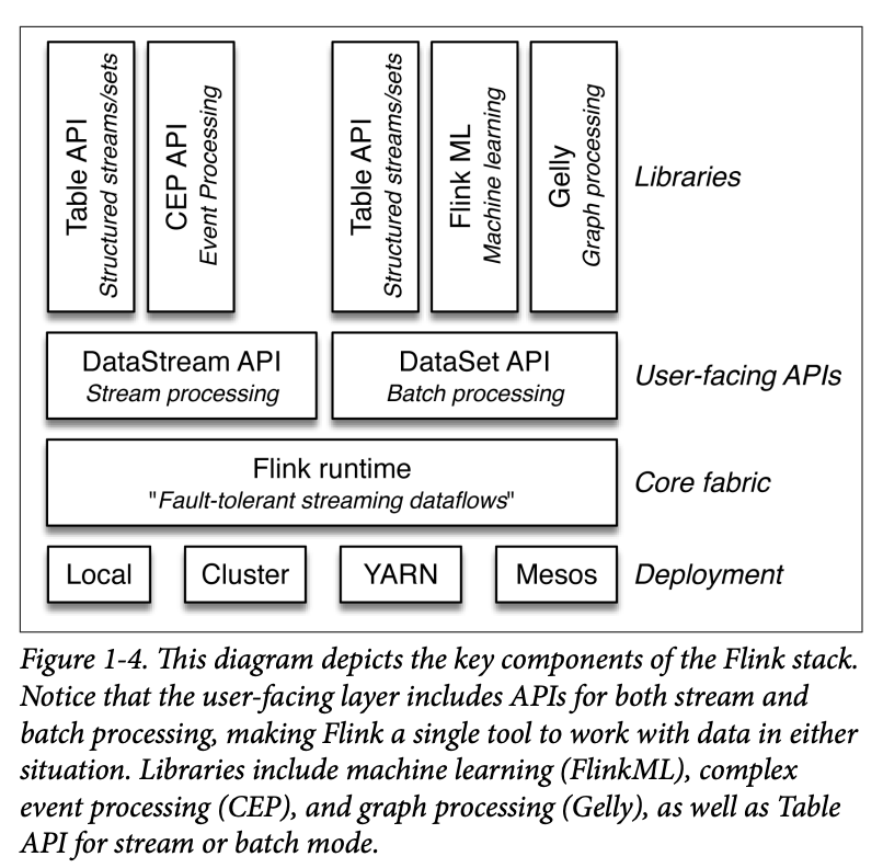
Programs accepted by the runtime are very powerful, but are verbose and difficult to program directly. For that reason, Flink offers developer-friendly APIs that layer on top of the runtime and generate these streaming dataflow programs. There is the DataStream API for stream processing and a DataSet API for batch processing.

Flink is distributed in the sense that it can run on hundreds or thou‐ sands of machines, distributing a large computation in small chunks, with each machine executing one chunk. The Flink frame‐ work automatically takes care of correctly restoring the computation in the event of machine and other failures, or intentional reprocessing, as in the case of bug fixes or version upgrades. This capability alleviates the need for the programmer to worry about failures.

Stream-First Architecture

Traditional Architecture versus Streaming Architecture

Traditionally, the typical architecture of a data backend has employed a centralized database system to hold the transactional data of the business. In other words, the database (be that a SQL or NoSQL) holds the “fresh” data, which represents the state of the business right now.

This might, for example, mean how many users are logged in to your system, how many active users a website has, or what the current balance of each user account is. Data applications that need fresh data are implemented against the database.

This traditional architecture has served applications well for decades, but is now being strained under the burden of increasing complexity in very large-scale distributed systems. Some of the main problems that companies have observed are:

• The pipeline from data ingestion to analytics is too complex and slow for many projects.
• The traditional architecture is too monolithic: the database backend acts as a single source of truth, and all applications need to access this backend for their data needs.

Another problem of this traditional architecture stems from trying to maintain the current “state of the world” consistently across a large, distributed system. At scale, it becomes harder and harder to maintain such precise synchronization; stream-first architectures allow us to relax the requirements so that we only need to maintain much more localized consistency.

A modern alternative approach, streaming architecture, solves many of the problems. In a stream-based design, we take this a step further and let data records continuously flow from data sources to applications and between applications.

There is no single database that holds the global state of the world. Rather, the single source of truth is in shared, ever-moving event streams—this is what represents the history of the business. In this stream-first architecture, applications themselves build their local views of the world, stored in local databases, distributed files, or search documents, for instance.

Message Transport and Message Processing

What is needed to implement an effective stream-first architecture and to gain the advantages of using Flink? 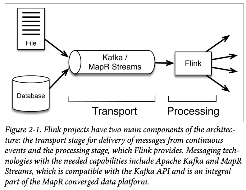A common pattern is to implement a streaming architecture by using two main kinds of components, represented in Figure 2-1:

1. A message transport to collect and deliver data from continuous events from a variety of sources (producers) and send this to applications that subscribe to it (consumers).
2. A stream processing system to (1) consistently move data between applications, (2) aggregate and process events, and (3) maintain local application state (again consistently).

The Transport Layer: Ideal Capabilities

What are the capabilities needed by the message transport system in streaming architecture?

Performance with Persistence

One of the roles of the transport layer is to serve as a safety queue upstream from the processing step—a buffer to hold event data as a kind of short-term insurance against an interruption in processing as data is ingested.

A key benefit of a persistent transport layer is that messages are replayable. This key capability allows a data processor like Flink to replay and recompute a specified part of the stream of events (discussed in further detail in Chapter 5).

For now, the key is to recognize that it is the interplay of transport and processing that allows a system like Flink to provide guarantees about correct processing and to do “time travel,” which refers to the ability to reprocess data.

Decoupling of Multiple Producers from Multiple Consumers

An effective messaging technology enables collection of data from many sources (producers) and makes it available to multiple application (consumers), as depicted in Figure 2-2. 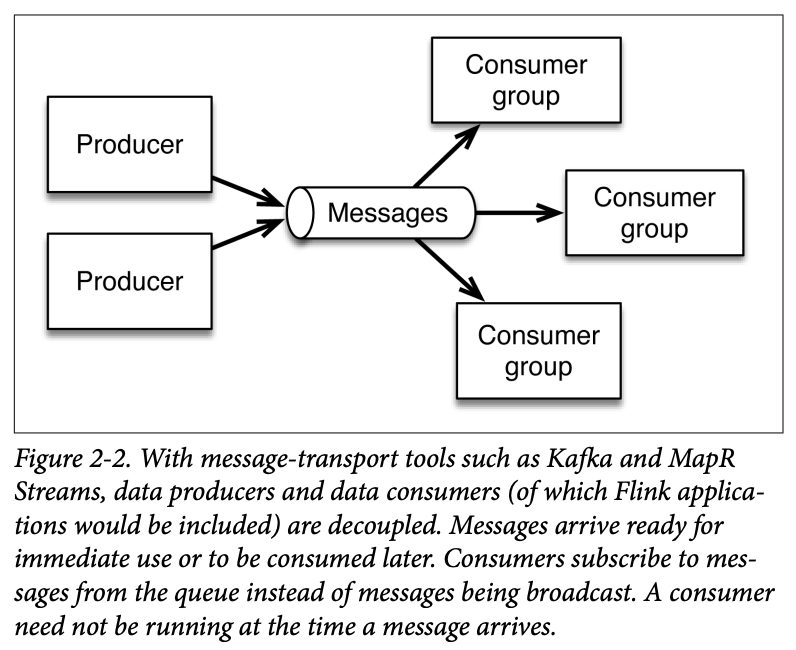With Kafka and MapR Streams, data from producers is assigned to a named topic. Data sources push data to the message queue, and consumers (or consumer groups) pull data. Event data can only be read forward from a given offset in the message queue.

Producers do not broadcast to all consumers automatically. This may sound like a small detail, but this characteristic has an enormous impact on how this architecture functions.

This style of delivery—with consumers subscribing to their topics of interest—means that messages arrive immediately, but they don’t need to be processed immediately. Consumers don’t need to be running when the messages arrive; they can make use of the data any time they like.

Having a message-transport system that decouples producers from consumers is powerful because it can support a microservices approach and allows processing steps to hide their implementations, and thus provides them with the freedom to change those implementations.

Data Stream as the Centralized Source of Data

Now you can put together these ideas to envision how message transport queues interconnect various applications to become, essentially, the heart of the streaming architecture. The stream processor (Flink, in our case) subscribes to data from the message queues and processes it. The output can go to another message transport queue. That way other applications, including other Flink applications, have access to the shared streaming data. In some cases, the output is stored in a local database. This approach is depicted in Figure 2-3. 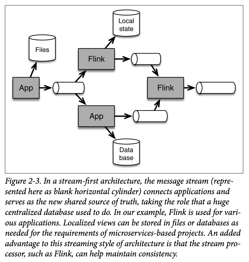In the streaming architecture, there need not be a centralized database. Instead, the message queues serve as a shared information source for a variety of different consumers.

What Flink does

SKIP

Handling Time

One crucial difference between programming applications for a stream processor and a batch processor is the need to explicitly handle time.

Let us take a very simple application: counting. We have a never-ending stream of events coming in (e.g., tweets, clicks, transactions), and we want to group the events by a key, and periodically (say, every hour) output the count of the distinct events for each key.

This is the proverbial application for “big data” that is analogous to the infamous word-counting example for MapReduce.

Counting in Batch/Lambda Architecture

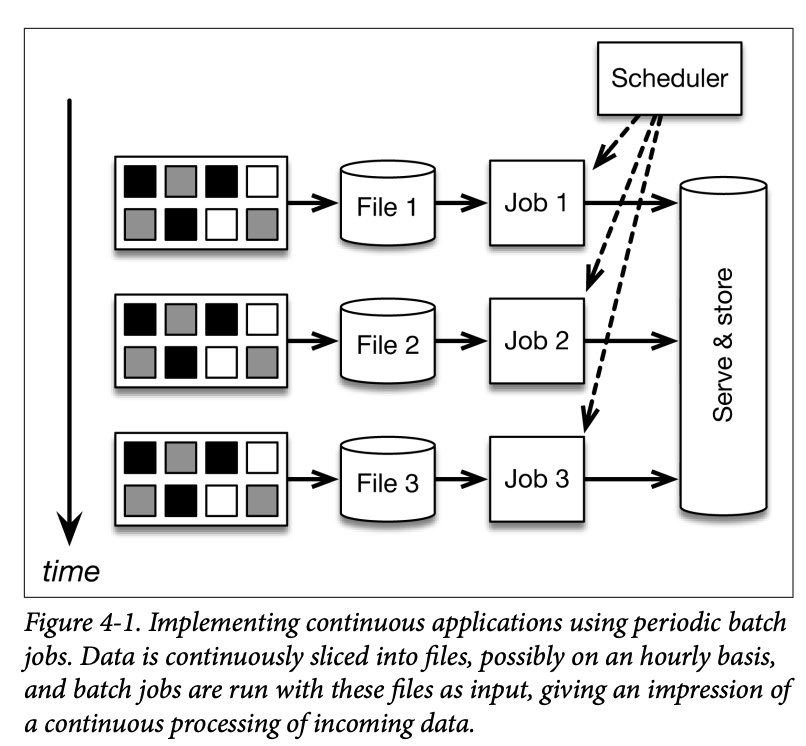In this architecture, a continuous data ingestion pipeline creates files (typically stored in a distributed file store such as HDFS every hours. This can be done by using a tool like Apache Flume. A batch job (using MapReduce or some alternative such as Apache Spark) is scheduled by a scheduler(such as Apache Airflow) to analyze the last file produced—grouping the events in the file by key, and counting distinct events per key—to output the last counts. Every company that is using Hadoop has several pipelines like this running in their clusters.

Although this architecture can certainly be made to work, there are several problems with it:

• Too many moving parts: We are using a lot of systems to count events in our incoming data. All of these come with their learn‐ ing and administration costs as well as bugs in all of the differ‐ ent programs.
• Early alerts: Let’s say that we want to get early count alerts ASAP (when receiving, say, at least 10 events), in addition to counting every one hour. For that, we can use Storm to ingest the message stream (Kafka or MapR Streams) in addition to the periodic batch jobs. We just added yet another system to the mix, along with a new programming model. This is called the Lambda architecture, described briefly in Chapter 1 and shown here in Figure 4-2.
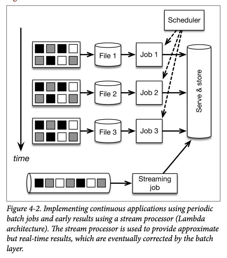
• Unclear batch boundaries: The meaning of “hourly” is kind of ambiguous in this architecture, as it really depends on the interaction between different systems. Cutting the data stream into hourly batches is actually the simplest possible way to divide time. Assume that we would like to produce aggregates, not for simple hourly batches, but instead for sessions of activity (e.g., from login until logout or inactivity). There is no straightforward way to do this in lambda architecture.

Counting in Streaming Architectures

There surely must be a better way to produce counts from a stream of events. As you might have suspected already, this is a streaming architecture. Using a streaming architecture, the application would follow the model in Figure 4-3.

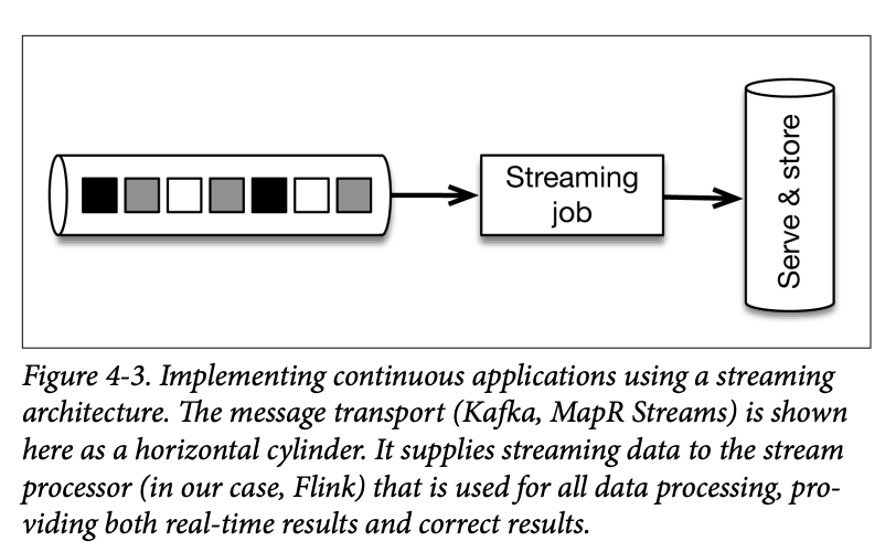
The event stream is again served by the message transport and simply consumed by a single Flink job that produces hourly counts and (optional) early alerts. This approach solves all the previous problems in a straightforward way.

• Slowdowns in the Flink job or throughput spikes simply pile up in the message-transport tool.
• The logic to divide events into timely batches (called windows) is embedded entirely in the application logic of the Flink program.
• Early alerts are produced by the same program.
• Out-of-order events are transparently handled by Flink. Grouping by session instead of a fixed time means simply changing the window definition in the Flink program. Additionally, replaying the application with changed code means simply replaying the Kafka topic.
• By adopting a streaming architecture, we have vastly reduced the number of systems to learn, administer, and create code in. The Flink application code to do this counting is straightforward:

DataStream stream = env                   
	.addSource(new FlinkKafkaConsumer(...))  // create stream from Kafka 
	.keyBy("country")                        // group by country 
	.timeWindow(Time.minutes(60))            // window of size 1 hour 
	.apply(new CountPerWindowFunction());    // do operations per window 

There are two main differences between the two approaches:

1. we are treating the never-ending stream of incoming events as what it actually is—a stream—rather than trying to artificially cut it into files,
2. we are explicitly encoding the definition of time (to divide the stream into groups) in the application code (the time window above) instead of implicitly spreading its definition to ingestion, computation, and scheduling.

Notions of Time

In stream processing, we generally speak about two main notions of time:

• Event time is the time that an event actually happened in the real world. More accurately, each event is usually associated with a timestamp that is part of the data record itself (e.g., as measured by a mobile phone or a server that emits logs). The event time of an event is simply a timestamp.
• Processing time is the time that the event is observed by the machine that is processing it. The processing time of an event is simply the time measured by the clock of the machine that is processing the event.

Event time is crucial when processing events in the correct chronological order, regardless of when they are processed by the system. For example, if you’re analyzing logs from multiple servers, you want to sort them by the time the events occurred, not by the time they were processed.

Processing time is used when the system’s response time is critical and you want to react to events as they arrive, regardless of their actual occurrence time. It’s often used in monitoring and alerting systems where you need to act on data as soon as it’s received.

See more on Event Time vs. Processing Time

Windowing

In the first section of this chapter, we reviewed an example of defining a time window in Flink, to aggregate the results of the last hour. Windows are the mechanism to group and collect a bunch of events by time or some other characteristic in order to do some analysis on these events as a whole (e.g., to sum them up)

Time Window

The simplest and most useful form of windows are those based on time. Time windows can be tumbling or sliding. For example, assume that we are counting the values emitted by a sensor and compare these choices.

Tumbling Window

A tumbling window of 1 minute collects the values of the last minute, and emits their sum at the end of the minute, as shown in Figure 4-5.

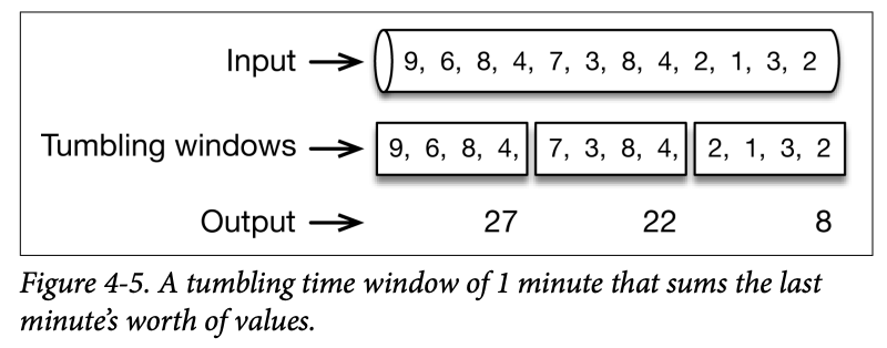
A tumbling time window of 1 minute can be defined in Flink simply as:

stream.timeWindow(Time.minutes(1))

Sliding Window

A sliding window of 1 minute that slides every half minute counts the values of the last minute, emitting the count every half minute, as shown in Figure 4-6. 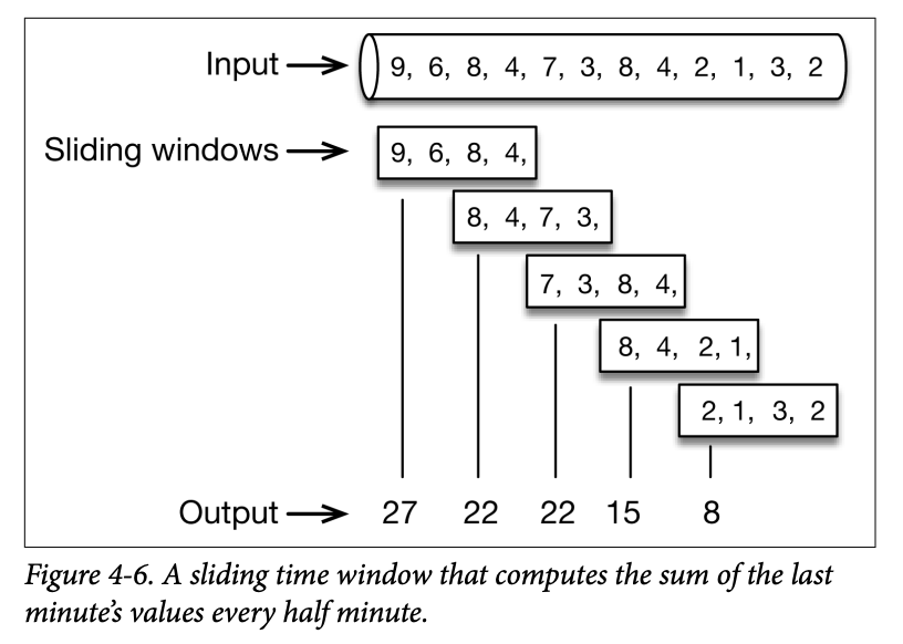A sliding time window of 1 minute that slides every 30 seconds can be defined as simply as:

stream.timeWindow(Time.minutes(1), Time.seconds(30))

Count Window

Another common type of window supported by Flink is the count window. Here, we are grouping elements based on their counts instead of timestamps. For example, the sliding window in Figure 4-6 can also be interpreted as a count window of size 4 elements that slides every 2 elements. Tumbling and sliding count windows can be defined as simply as:

stream.countWindow(4)
stream.countWindow(4, 2)

Count windows, while useful, are less rigorously defined than time windows and should be used with care.

Because time always goes on, a time window will always eventually “close.” However, with a count window of, say, 100 elements, you might have a situation where there are never 100 elements for this key, which will lead to the window never closing, and the memory occupied by the window will remain garbage.

One way to mitigate that is to couple a time window with a timeout using a trigger, which we will describe later in the section “Triggers”.

Session

Another very useful type of window provided by Flink is the session window.

A session is a period of activity that is preceded and followed by a period of inactivity; for example, a series of interactions of a user on a website, followed by the user closing the browser tab or simply becoming inactive.

Sessions need their own mechanism because they typically do not have a set duration (some sessions can be 30 seconds and another 1 hour), or a set number of interactions (some sessions can be 3 clicks followed by a purchase and another can be 40 clicks without a pur‐ chase).

Session windows in Flink are specified using a timeout. This basically specifies how long we want to wait until we believe that a session has ended. For example, here we expire a session when the user is inactive for five minutes:

stream.window(SessionWindows.withGap(Time.minutes(5))

Trigger

In addition to windows, Flink also provides an optional mechanism to define triggers.

Triggers control when the results are made available—in other words, when the contents of a window will be aggregated and returned to the user.

Every default window comes coupled with a trigger. For example, a time window on event time is triggered when a watermark arrives. But as a user, you can also implement a custom trigger (for example, providing approximate early results of the window every 1 second) in addition to the complete and accurate results when the watermark arrives.

Time Travel

An aspect central to the streaming architecture is time travel. If all data processing is done by the stream processor, then how do we evolve applications, how do we process historical data, and how do we reprocess the data (say, for debugging or auditing purposes)? 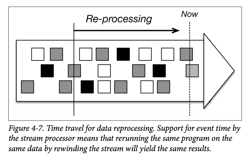As shown in Figure 4-7, time travel means rewinding the stream to some time in the past and restarting the processing from there, eventually catching up with the present.

If windows are defined based on wall-clock time instead of the timestamps embedded in the records themselves, every time we run the same application, we will get a different result. Event time makes processing deterministic by guaranteeing that running the same application on the same stream will yield the same results.

Watermarks

Background

We saw that support for event time is central to the streaming architecture, providing accuracy and the ability to reprocess data.

When computation is based on event time, how do we know that all events have arrived, and that we can compute and output the result of a window? In other words, how do we keep track of event time and know that a certain event time has been reached in the input stream?

To keep track of event time, we need some sort of clock that is driven by the data instead of the wall clocks of the machines performing the computation.

Consider the 1-minute tumbling windows of Figure 4-5. Assume that the first window starts at 10:00:00 and needs to sum up all values from 10:00:00 until 10:01:00. How do we know that the time is 10:01:00 when time is part of the records themselves? In other words, how do we know that an element with timestamp 10:00:59 will not arrive?

Introduction to Watermark

Flink achieves this via watermarks, a mechanism to advance event time. Watermarks are regular records embedded in the stream that, based on event time, inform computations that a certain time has been reached.

When the aforementioned window receives a watermark with a time marker greater than 10:01:00 (for example, both a watermark with time marker 10:01:00 and a watermark with time marker 10:03:43 would work the same), it knows that no further records with a timestamp greater than the marker will occur; all events with time less than or equal to the timestamp have already occurred. It can then safely compute and emit the result of the window (the sum).

With watermarks, event time progresses completely independently from processing time. For example, if a watermark is late (“late” being measured in processing time), this will not affect the correctness of the results, only the speed in which we get the results.

How to generate Watermark

In Flink, the application developer generates watermarks, as doing so usually requires some knowledge of the domain. A perfect watermark is a watermark that can never be wrong; that is, no event will ever arrive after a watermark with an event time from before the watermark.

Domain knowledge is often used to specify a watermark. For exam‐ ple, we may know that our events might be late, but cannot possibly be more than five seconds late, which means that we can emit a watermark of the largest timestamp seen, minus five seconds. Or, a different Flink job may monitor the stream and construct a model for generating watermarks, learning from the lateness of the events as they arrive.

If watermarks are too slow, we might see a slowdown in the speed with which we are getting output, but we can remedy that by emitting approximate results even before the watermark (Flink provides mechanisms for doing so).

If watermarks are too fast, we might get a result that we think is correct but is not, and we can remedy that by using Flink’s mechanisms for late data.

If all of this seems complicated, remember that most event streams in the real world are out of order and that there is no such thing (usually) as perfect knowledge about how out of order they are. (In theory, we would have to look at the future for that.)

Watermarks are the only mechanism that require us to deal with out-of-order data and to bound the correctness of our results; the alternative would be ignoring reality and pretending that our results are correct when they are not, without any bounds on their correctness.

TODO read:

• https://medium.com/@ipolyzos_/understanding-watermarks-in-apache-flink-c8793a50fbb8
• https://nightlies.apache.org/flink/flink-docs-master/docs/dev/datastream/event-time/generating_watermarks/
• https://medium.com/@detwk/unraveling-the-mystery-of-watermarks-in-apache-flink-an-internal-perspective-a4738bf4f561

Stateful Computation

Streaming computation can be either stateless or stateful.

A stateless program looks at each individual event and creates some output based on that last event. For example, a streaming program might receive temperature readings from a sensor and raise an alert if the temperature goes beyond 90 degrees.

A stateful program creates out‐ put based on multiple events taken together. Examples of stateful programs include:

• All types of windows that we discussed in Chapter 4. For example, getting the average temperature reported by a sensor over the last hour is a stateful computation.
• All kinds of state machines used for complex event processing (CEP).
• For example, creating an alert after receiving 2 temperature readings that differ by more than 20 degrees within 1 minute is a stateful computation.
• All kinds of joins between streams as well as joins between streams, and static or slowly changing tables. 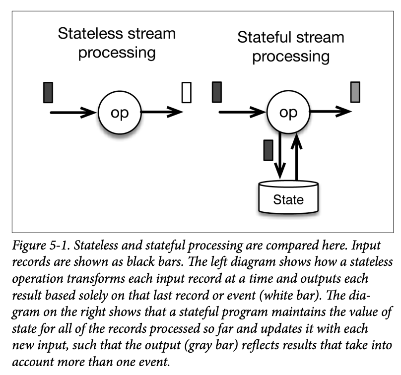Figure 5-1 exemplifies the main difference between stateless and stateful stream processing.

A stateless program receives each record separately (black input) and produces each output record based on the last input record alone (white records).

A stateful program maintains state that is updated based on every input and produces output (gray records) based on the last input and the current value of the state.

Notions of Consistency

In the terminology of the stream processing world, people distinguish between three different levels of consistency:

• At-most once: the count may be lost after a failure
• At-least once: the count may be bigger than but never smaller than the correct count
• Exactly once: the count will be exactly the same as it would be in the failure-free scenario See more: Message Delivery Guarantee

It used to be that at least once was very popular in the industry, with the first stream processors (Apache Storm, Apache Samza) guaranteeing only at least once when they first came out. This was the case for two reasons:

1. It is trickier to implement systems that guarantee exactly once. Exactly once is challenging at both the fundamental level (to decide what correct means exactly), and at the implementation level.
2. Early adopters of stream processing were willing to work around the framework limitations at the application level (e.g., by making their applications idempotent.

The first solutions that provided exactly once (Trident, Spark Streaming) came at a substantial cost in terms of performance and expressiveness. In order to guarantee exactly once behavior, these systems do not apply the application logic to each record separately, but instead process several (a batch of) records at a time, guaranteeing that either the processing of each batch will succeed as a whole or not at all. This situation implies that you have to wait for a batch to complete before getting any results.

Essentially, Flink eliminates these tradeoffs by allowing a single framework to handle all requirements, a meaningful technological leap in the industry, which, like all such leaps, seems magical from the outside but makes a lot of sense when explained.

Flink Checkpoints: Guaranteeing Exactly Once

How does Flink guarantee exactly once processing? Flink makes use of a feature known as “checkpoints” as a way to reset to the correct state in the case of a failure.

Checkpointing allows Flink to periodically take snapshots of the state of the application, which can be used to restore the application to a correct state in the event of a failure.

Checkpointing Mechanism

• Flink periodically takes snapshots of the state of operators in the data flow graph.
• These snapshots are stored in a persistent storage like HDFS, S3, or any other reliable storage system.
• When a failure occurs, Flink can recover the state of the application from the last successful checkpoint, allowing it to reprocess the data starting from that point.

Barrier

• Flink injects special records called “barriers” into the data stream.
• These barriers flow through the data stream and, when they reach an operator, they signal the operator to take a snapshot of its state.
• The barriers ensure that all records before the barrier have been processed, and all records after it belong to the next checkpoint.

State Backend

Flink uses state backends to store and manage the state. The two main state backends are:

1. The Heap-based State Backend (which stores state in the JVM heap)
2. The RocksDB State Backend (which stores state in RocksDB).

Transactionally Writing Output

• For exactly-once semantics, the sinks (where the output is written) must also support exactly-once guarantees.
• For example, when writing to Kafka, Flink uses the Kafka Producer’s transactional API to commit offsets only after a checkpoint has been successfully completed.

Savepoints: Versioning State

Previously, we saw that checkpoints are automatically generated by Flink to provide a way to reprocess records while correcting state in case of a failure. But Flink users also have a way to consciously manage versions of state through a feature called savepoints.

A savepoint is taken in exactly the same way as a checkpoint but is triggered manually by the user (using the Flink CLI tools or the web console) instead of by Flink itself. Like checkpoints, savepoints are also stored in stable storage and give the user the ability to start a new version of the job or to restart the job from a savepoint rather than from a beginning in time. You can think of savepoints as snapshots of a job at a certain time.

You can use savepoints to solve a variety of production issues for streaming jobs:

1. Application code upgrades: Assume that you have found a bug in an already running application and you want the future events to be processed by the updated code with the bug fixed. By tak‐ ing a savepoint of the job and restarting from that savepoint using the new code, downstream applications will not see the difference (except for the update of course).
2. Flink version upgrades: Upgrading Flink itself also becomes easy because you can take savepoints of running pipelines and replay them from the savepoints using an upgraded Flink version
3. Maintenance and migration: Using savepoints, you can easily “pause and resume” an application. This is especially useful for cluster maintenance as well as migrating jobs consistently to a new cluster.
4. What-if simulations (reinstatements): Many times, it is very use‐ ful to run an alternative application logic to model “what-if ” scenarios from controllable points in the past.
5. A/B testing: By running two different versions of application code in parallel from the exact same savepoint, you can model A/B testing scenarios.

Conclusion

In this chapter, we saw how stateful stream processing changes the rules of the game.

By having checkpointed state as a first-class citizen inside the stream processor, we can get correct results after failures, very high throughput, and low latency all at the same time, completely eliminating past tradeoffs that people thought of as fundamental (but are not). This is one of the most important advantages of Flink.

Another advantage of Flink is its ability to handle streaming and batch using a single technology, completely eliminating the need for a dedicated batch layer. Chapter 6 provides a brief overview of how batch processing with Flink is possible.

Batch is a Special Case of Streaming

SKIP